Pandas Applications and Regression Preview

강의자료 다운로드: click me

Learning Objectives

Pandas Application
- Grouping, Combining
- Pivoting, Reshaping
- Custom Functions
Working with Database using Pandas
- SQLite
- Create/Load/Handing DB
Regression Preview
- Using Numpy
- Using Scikit-learn

Pandas Applications

Pandas is one of the most powerful and widely used Python libraries for data analysis. Beyond basic operations such as loading CSV files or selecting rows and columns, Pandas provides advanced functionalities that make it suitable for real-world applications.

These applications help researchers, data scientists, and engineers handle large datasets, transform them into meaningful structures, and prepare them for further machine learning tasks.

Grouping and Aggregation With functions like groupby and agg, Pandas allows us to summarize data based on categories. For example, we can compute the average salary per department, the total sales per region, or the maximum score per student group.
Combining Data Real-world data is often split across multiple tables. Pandas provides merge, concat, and join functions to combine datasets seamlessly. This resembles SQL joins and is essential when integrating information from different sources.
Pivoting and Reshaping Using pivot, pivot_table, and melt, Pandas can reshape datasets into more convenient formats. This is especially useful for producing summary tables or preparing data for visualization and statistical modeling.
Applying Custom Functions Pandas integrates well with Python functions. The apply method and lambda expressions allow us to create new variables, transform existing ones, and apply complex logic to entire datasets with minimal code.
Working with Databases Pandas can directly interact with relational databases such as SQLite, MySQL, or PostgreSQL. This allows us to read tables into DataFrames, perform transformations in Python, and save the results back to the database. It is especially useful when datasets are too large to handle with plain CSV or Excel files.

In practice, these applications make Pandas more than just a data manipulation tool. They transform it into a bridge between raw data and meaningful analysis, enabling us to prepare datasets effectively before applying machine learning algorithms.

Grouping and Aggregation

In many data analysis tasks, we need to group data by categories and compute summary statistics. Pandas provides the groupby method along with agg to calculate measures such as mean, sum, or standard deviation for each group.

What is `groupby()`?

groupby() is a powerful method in Pandas used to split a DataFrame into groups based on one or more keys (columns).

It is conceptually similar to the GROUP BY clause in SQL.

Key Idea

It groups data but does not calculate anything by itself.
It returns a DataFrameGroupBy object, which represents grouped data ready for aggregation or transformation.

Basic Example

df.groupby("Genre")

This creates a grouped object but does not perform any computation yet.

You can iterate through groups to inspect them:

for name, group in df.groupby("Genre"):
    print("Group:", name)
    print(group.head(2))

Explanation:

name: the group key (e.g., 'Rock', 'Jazz', 'Pop')
group: a smaller DataFrame containing only the rows for that category.

Pandas `groupby` with Multiple Columns

Concept Overview

groupby(["col1", "col2", ...]) groups data based on combinations of multiple columns (multi-key grouping).
Each unique combination of values forms one group.
By default, the result uses a MultiIndex, but you can set as_index=False to return a flat DataFrame.

Basic Example

import pandas as pd

data = {
    "Country": ["USA", "USA", "Canada", "USA", "Canada", "Canada"],
    "Genre":   ["Rock","Pop", "Rock", "Rock","Jazz",  "Rock"],
    "Year":    [2023, 2023,   2023, 2024,   2023,     2024],
    "Revenue": [10,   15,     8,    12,     7,       6]
}
df = pd.DataFrame(data)
df

	Country	Genre	Year	Revenue
0	USA	Rock	2023	10
1	USA	Pop	2023	15
2	Canada	Rock	2023	8
3	USA	Rock	2024	12
4	Canada	Jazz	2023	7
5	Canada	Rock	2024	6

Grouping by Multiple Columns + Single Aggregation

# Sum of Revenue by Country and Genre
out = df.groupby(["Country", "Genre"])["Revenue"].sum()
out

Country  Genre
Canada   Jazz      7
         Rock     14
USA      Pop      15
         Rock     22
Name: Revenue, dtype: int64

Using as_index=False for a flat table

out_flat = (
    df.groupby(["Country", "Genre"], as_index=False)["Revenue"]
      .sum()
      .sort_values(["Country", "Genre"])
)
out_flat

Country	Genre	Revenue
Canada	Jazz	7
Canada	Rock	14
USA	Pop	15
USA	Rock	22

Applying Aggregation with `agg()`

The agg() (aggregate) function is used to summarize data by applying one or more statistical functions to each group.

Basic Usage

df.groupby("Genre")["Revenue"].agg(["sum", "mean", "std"])

This computes the sum, mean, and standard deviation of the Revenue column for each Genre.

Different Functions for Different Columns

df.groupby("Genre").agg({
    "Revenue": ["sum", "mean"],
    "Price": "max"
})

You can pass a dictionary to specify different aggregation functions for each column.

Without `groupby()`

You can also use agg() directly on a DataFrame:

df.agg(["mean", "sum", "max"])

→ Computes the statistics across all numeric columns.

Custom Aggregation

You can define custom functions using lambda:

df.agg({
    "Sales": lambda x: x.max() - x.min(),
    "Profit": "mean"
})

This calculates the range for Sales and the average for Profit.

Exercise

# Create a DataFrame with teams and performance data
data = {
    "team": ["A","A","B","B","C","C","A","B","C","A"],
    "score": [85,90,78,88,95,92,89,84,91,87],
    "hours": [5,6,4,5,7,6,8,3,4,7]
}
df = pd.DataFrame(data)

# Group data by team and calculate mean and standard deviation
result = df.groupby("team").agg({"score":"mean", "hours":"std"})
print(result)

- Results

          score     hours
team                     
A     87.750000  1.290994
B     83.333333  1.000000
C     92.666667  1.527525

Combining DataFrames

Real-world datasets often come from multiple sources.

Pandas offers several ways to combine DataFrames:

merge: SQL-style join on keys
concat: Concatenate DataFrames along rows or columns
join: Merge DataFrames by index

`merge()`

Concept

merge() is similar to SQL's JOIN operation.

It combines rows from two DataFrames based on one or more common key columns.

Basic Syntax

pd.merge(left, right, on="key", how="inner")

Parameter	Description
`left`, `right`	DataFrames to be merged
`on`	Column name(s) to join on
`how`	Type of join: `'inner'`, `'left'`, `'right'`, `'outer'`

Example

import pandas as pd

employees = pd.DataFrame({
    "EmpID": [1, 2, 3, 4],
    "Name": ["Alice", "Bob", "Charlie", "David"]
})

departments = pd.DataFrame({
    "EmpID": [2, 4, 5],
    "Dept": ["Sales", "HR", "IT"]
})

pd.merge(employees, departments, on="EmpID", how="inner")

Result (INNER JOIN):

EmpID	Name	Dept
2	Bob	Sales
4	David	HR

Join Types

Type	Description
`inner`	Keeps only matching keys (default)
`left`	Keeps all from left, adds matching from right
`right`	Keeps all from right, adds matching from left
`outer`	Keeps all keys, fills missing values with NaN

`concat()`

Concept

concat() is used to stack DataFrames either vertically (row-wise) or horizontally (column-wise).

Basic Syntax

pd.concat([df1, df2], axis=0, ignore_index=True)

Parameter	Description
`axis=0`	Stack rows (default)
`axis=1`	Stack columns
`ignore_index=True`	Reset the index in the result

Example — Row-wise Concatenation

df1 = pd.DataFrame({"A": [1, 2], "B": [3, 4]})
df2 = pd.DataFrame({"A": [5, 6], "B": [7, 8]})
pd.concat([df1, df2], axis=0, ignore_index=True)

Result:

A	B
1	3
2	4
5	7
6	8

Example — Column-wise Concatenation

pd.concat([df1, df2], axis=1)

Result:

A	B	A	B
1	3	5	7
2	4	6	8

`join()`

Concept

join() merges two DataFrames using their index rather than columns.

Basic Syntax

df1.join(df2, how="left")

Parameter	Description
`how`	Type of join: `'left'`, `'right'`, `'outer'`, `'inner'`
`on`	Column to join on (optional if indexes align)

Example

df1 = pd.DataFrame({"A": [1, 2, 3]}, index=["x", "y", "z"])
df2 = pd.DataFrame({"B": [10, 20, 30]}, index=["y", "z", "w"])
df1.join(df2, how="outer")

Result:

index	A	B
x	1	NaN
y	2	10
z	3	20
w	NaN	30

When to Use Each Method

Method	Purpose	Join Basis	Typical Use Case
`merge()`	SQL-style joins	Column keys	Combine data by ID or key
`concat()`	Append or stack data	Axis (row/column)	Combine datasets of same schema
`join()`	Merge by index	Index	Combine aligned DataFrames (e.g., time series)

Practical Tips

Operation	Works Like	Aligns On	Output Example
`merge()`	SQL JOIN	Keys (columns)	Match records
`concat()`	UNION / STACK	Row or column axis	Combine datasets
`join()`	SQL JOIN on index	Index	Combine by row labels

Excercise

import pandas as pd

# -----------------------------
# Sample DataFrames
# -----------------------------
df1 = pd.DataFrame({
    "id": [1, 2, 3, 4, 5],
    "name": ["Kim", "Lee", "Park", "Choi", "Jung"]
})
df2 = pd.DataFrame({
    "id": [1, 2, 3, 4, 5],
    "score": [90, 85, 88, 92, 75]
})

# ============================================================
# 1) MERGE — SQL-style join on one or more key columns
# ============================================================
# `pd.merge(left, right, on=None, how='inner')`
# ------------------------------------------------------------
# - `on`: column name(s) used as key(s) to join on.
# - `how`: join type. Options:
#       "inner" → keep only matching keys (default)
#       "left"  → keep all rows from the left DataFrame
#       "right" → keep all rows from the right DataFrame
#       "outer" → keep all keys from both (union)
# - `suffixes`: add suffixes when non-key columns overlap
# ============================================================

merged_inner = pd.merge(
    df1,
    df2,
    on="id",
    how="inner"
)
print("MERGE (inner join on 'id'):\n", merged_inner, "\n")

merged_left = pd.merge(
    df1,
    df2,
    on="id",
    how="left"
)
print("MERGE (left join on 'id'):\n", merged_left, "\n")

merged_outer = pd.merge(
    df1,
    df2,
    on="id",
    how="outer"
)
print("MERGE (outer join on 'id'):\n", merged_outer, "\n")

# ============================================================
# 2) CONCAT — Stack DataFrames vertically or horizontally
# ============================================================
# `pd.concat(objs, axis=0, ignore_index=False)`
# ------------------------------------------------------------
# - `axis=0`: stack along rows (default)
# - `axis=1`: combine columns side-by-side
# - `ignore_index=True`: reset index after concatenation
# ============================================================

concat_cols = pd.concat(
    [df1, df2],
    axis=1
)
print("CONCAT (axis=1 — columns):\n", concat_cols, "\n")

df_more = pd.DataFrame({
    "id": [6, 7],
    "score": [80, 77]
})
concat_rows = pd.concat(
    [df2, df_more],
    axis=0,
    ignore_index=True
)
print("CONCAT (axis=0 — rows, ignore_index=True):\n", concat_rows, "\n")

# ============================================================
# 3) JOIN — Merge by index (can use 'on' for left DataFrame)
# ============================================================
# `DataFrame.join(other, on=None, how='left')`
# ------------------------------------------------------------
# - Joins two DataFrames based on their **index**.
# - If `on` is given, use that column from the left DataFrame
#   and match it to the index of the right DataFrame.
# - `how` options:
#       "left"  → keep all left rows (default)
#       "inner" → keep only intersection of index keys
#       "outer" → keep all index keys (union)
#       "right" → keep all right rows
# ============================================================

right_indexed = df2.set_index("id")

# LEFT JOIN: keep all rows from df1
joined_left = df1.join(
    right_indexed,
    on="id",
    how="left"
)
print("JOIN (how='left', on='id'):\n", joined_left, "\n")

# INNER JOIN: keep only ids present in both
joined_inner = df1.join(
    right_indexed,
    on="id",
    how="inner"
)
print("JOIN (how='inner', on='id'):\n", joined_inner, "\n")

# OUTER JOIN: include all ids from both DataFrames
df2_extra = pd.DataFrame({
    "id": [5, 6],
    "score": [75, 99]
}).set_index("id")

joined_outer = df1.join(
    df2_extra,
    on="id",
    how="outer"
)
print("JOIN (how='outer', on='id') — with extra id=6:\n", joined_outer, "\n")

# JOIN by index on both sides
df1_indexed = df1.set_index("id")
df2_indexed = df2.set_index("id")

joined_index = df1_indexed.join(
    df2_indexed,
    how="inner"
)
print("JOIN by index (how='inner'):\n", joined_index, "\n")

Results

MERGE (inner join on 'id'):
    id  name  score
0   1   Kim     90
1   2   Lee     85
2   3  Park     88
3   4  Choi     92
4   5  Jung     75 

MERGE (left join on 'id'):
    id  name  score
0   1   Kim     90
1   2   Lee     85
2   3  Park     88
3   4  Choi     92
4   5  Jung     75 

MERGE (outer join on 'id'):
    id  name  score
0   1   Kim     90
1   2   Lee     85
2   3  Park     88
3   4  Choi     92
4   5  Jung     75 

CONCAT (axis=1 — columns):
    id  name  id  score
0   1   Kim   1     90
1   2   Lee   2     85
2   3  Park   3     88
3   4  Choi   4     92
4   5  Jung   5     75 

CONCAT (axis=0 — rows, ignore_index=True):
    id  score
0   1     90
1   2     85
2   3     88
3   4     92
4   5     75
5   6     80
6   7     77 

JOIN (how='left', on='id'):
    id  name  score
0   1   Kim     90
1   2   Lee     85
2   3  Park     88
3   4  Choi     92
4   5  Jung     75 

JOIN (how='inner', on='id'):
    id  name  score
0   1   Kim     90
1   2   Lee     85
2   3  Park     88
3   4  Choi     92
4   5  Jung     75 

JOIN (how='outer', on='id') — with extra id=6:
      id  name  score
0.0   1   Kim    NaN
1.0   2   Lee    NaN
2.0   3  Park    NaN
3.0   4  Choi    NaN
4.0   5  Jung   75.0
NaN   6   NaN   99.0 

JOIN by index (how='inner'):
     name  score
id             
1    Kim     90
2    Lee     85
3   Park     88
4   Choi     92
5   Jung     75

Pivoting

Why pivot_table?

pivot_table reshapes and summarizes data, similar to Excel Pivot Tables.

It turns long/transactional data into a compact matrix for quick comparison (e.g., Revenue by Country and Genre).

Core Syntax

df.pivot_table(
    values=None,
    index=None,
    columns=None,
    aggfunc="mean",
    fill_value=None,
    margins=False,
    margins_name="All",
    dropna=True,
    observed=False
)

Key Parameters

values: Column(s) to aggregate (e.g., "Revenue"). If None, all numeric columns may be aggregated.
index: Row groups (one or more columns).
columns: Column groups (one or more columns).
aggfunc: Aggregation function(s), e.g., "sum", "mean", "count", np.sum, or a list/dict for multiple metrics.
fill_value: Replace NaN in the result with a value (commonly 0).
margins: Add row/column totals (True/False).
margins_name: Label for totals (default "All").
dropna: Drop columns in the result that are all-NaN.
observed: For categorical groupers, include only observed combinations (perf/size optimization).

Example 1. Average score per team

pivot_avg = df.pivot_table(
    values="score",
    index="team",
    aggfunc="mean"
)

Example 2. With Columns and Totals

# Average score by team (rows) and year (columns) + totals
pivot_avg_tc = df.pivot_table(
    values="score",
    index="team",
    columns="year",
    aggfunc="mean",
    margins=True,         # add totals
    margins_name="Total", # rename totals row/col
    fill_value=0          # replace NaN with 0 for display
)

Example 3. Multiple Aggregations

You can compute several statistics at once:

import numpy as np

pivot_multi = df.pivot_table(
    values="score",
    index="team",
    columns="year",
    aggfunc=["mean", "median", "count", np.std],
    fill_value=0
)

Example 4. Using Multiple Value Columns

Aggregate several value columns at once:

pivot_values = df.pivot_table(
    values=["score", "hours"],
    index="team",
    columns="year",
    aggfunc={"score": "mean", "hours": "sum"},
    fill_value=0
)

Exercise

import pandas as pd
import numpy as np

# ============================================================
# Create a Toy Dataset
# ============================================================
# We will create a simple DataFrame that contains team names,
# years, and corresponding scores. Each row represents one
# observation (a student's or team's score for a given year).
# ============================================================

df = pd.DataFrame({
    "team": ["A", "A", "B", "B", "C", "C"],
    "year": [2023, 2024, 2023, 2024, 2023, 2024],
    "score": [88, 92, 79, 85, 91, 87]
})

print("=== Original DataFrame ===")
print(df)
print("\n")

# ============================================================
# Example 1 — Average score per team
# ============================================================
# Goal:
# - Summarize the dataset by calculating the mean (average)
#   score for each team.
# - The 'team' column becomes the index (rows of the pivot table).
#
# Syntax:
#   df.pivot_table(values="score", index="team", aggfunc="mean")
#
# Parameters:
# - values: column to aggregate (e.g., 'score')
# - index: row-level grouping (e.g., 'team')
# - aggfunc: aggregation function ('mean', 'sum', 'count', etc.)
# ============================================================

pivot_avg = df.pivot_table(
    values="score",    # numeric column to aggregate
    index="team",      # group by 'team' (row grouping)
    aggfunc="mean"     # compute the mean (average)
)

print("=== Pivot Table: Average Score per Team ===")
print(pivot_avg)
print("\n")

# Explanation:
# Each row now represents a team, and the value shows
# the team's average score across all years.
# Equivalent operation using groupby:
# df.groupby("team")["score"].mean()

# ============================================================
# Example 2 — Average score by team and year (with totals)
# ============================================================
# Goal:
# - Create a 2D summary table that shows the average score
#   for each (team, year) combination.
# - Include totals for both rows and columns using `margins=True`.
#
# Syntax:
#   df.pivot_table(
#       values="score",
#       index="team",
#       columns="year",
#       aggfunc="mean",
#       margins=True,
#       margins_name="Total",
#       fill_value=0
#   )
#
# Parameters:
# - columns: defines column-level grouping (e.g., 'year')
# - margins: adds row/column totals (True or False)
# - margins_name: name for the totals row/column ('Total')
# - fill_value: replaces NaN with a chosen value (e.g., 0)
# ============================================================

pivot_avg_tc = df.pivot_table(
    values="score",       # numeric column to aggregate
    index="team",         # rows grouped by 'team'
    columns="year",       # columns grouped by 'year'
    aggfunc="mean",       # compute average per (team, year)
    margins=True,         # include totals for rows/columns
    margins_name="Total", # label the totals
    fill_value=0          # fill missing cells with 0
)

print("=== Pivot Table: Average Score by Team and Year ===")
print(pivot_avg_tc)
print("\n")

# Explanation:
# - Rows represent teams ('A', 'B', 'C', and 'Total').
# - Columns represent years (2023, 2024, and 'Total').
# - Each cell shows the average score for that combination.
# - The 'Total' row and column display overall averages.

# ============================================================
# Summary
# ============================================================
# Example 1 → One-dimensional summary (team-level averages)
# Example 2 → Two-dimensional summary (team × year matrix)
#
# Use pivot_table when you need to:
# - Summarize large datasets
# - Compare numeric metrics across multiple categories
# - Quickly create Excel-style summary tables within Python
# ============================================================

- Results

=== Original DataFrame ===
  team  year  score
0    A  2023     88
1    A  2024     92
2    B  2023     79
3    B  2024     85
4    C  2023     91
5    C  2024     87


=== Pivot Table: Average Score per Team ===
      score
team       
A      90.0
B      82.0
C      89.0


=== Pivot Table: Average Score by Team and Year ===
year   2023  2024  Total
team                    
A      88.0  92.0   90.0
B      79.0  85.0   82.0
C      91.0  87.0   89.0
Total  86.0  88.0   87.0

Working with Database Files

Pandas can work not only with CSV or Excel files but also with relational databases such as SQLite.

This is especially useful when data is stored in structured tables. By combining Pandas with the sqlite3 library, we can create a database, save a DataFrame into it, read data back with SQL queries, and update it after processing.

What is SQL (Structured Query Language)

SQL is a standard language used to manage and query relational databases.

It allows you to store, retrieve, and manipulate structured data efficiently.

Key SQL Operations

Operation	Keyword	Description
Create	`CREATE TABLE`	Define a new table
Insert	`INSERT INTO`	Add new records
Select	`SELECT ... FROM`	Retrieve data from tables
Update	`UPDATE ... SET`	Modify existing records
Delete	`DELETE FROM`	Remove records
Join	`JOIN`	Combine data from multiple tables

SQL Example

SELECT name, score
FROM students
WHERE score >= 90
ORDER BY score DESC;

Returns students who scored 90 or higher, sorted by score.

Why Learn SQL with Pandas?

SQL handles structured storage and querying
Pandas handles analysis, visualization, and modeling
Together: End-to-end data science workflow (data collection → SQL query → Pandas analysis)

Create a sample SQLite database file

This step demonstrates how to create a small database file and store a Pandas DataFrame inside it.

Instead of keeping all data in CSV or Excel files, we often need to use relational databases such as SQLite, which allow us to manage data more efficiently.

Pandas integrates seamlessly with SQLite through the sqlite3 module.

SQLite is a lightweight, serverless relational database engine.

Unlike large database systems (e.g., MySQL or PostgreSQL), SQLite does not require a separate server process.
Instead, it stores the entire database in a single file (e.g., sample.db).
This makes it very convenient for learning, prototyping, and handling small to medium-sized datasets.
Because it follows the SQL (Structured Query Language) standard, you can still use familiar SQL commands such as SELECT, INSERT, and UPDATE.

sqlite3 is the Python built-in module that lets you work with SQLite databases.

With sqlite3.connect("sample.db"), Python opens a connection to the database file.
If sample.db does not exist, it will be automatically created.
If the file already exists, it simply opens the existing database file.
You can then use this connection to run SQL queries or, in combination with Pandas, to store and retrieve DataFrames.

Note

Pandas can also connect to other relational databases such as MySQL and PostgreSQL.

Instead of sqlite3, you would typically use connectors such as pymysql (for MySQL) or psycopg2 (for PostgreSQL).
Combined with SQLAlchemy, Pandas can use the same read_sql() and to_sql() methods to read from or write to those databases as well.
This makes Pandas a very versatile tool for integrating with various database systems.

The workflow is:

Use Pandas to create a DataFrame with 10 rows of student data (ID, name, score).
Open a connection to sample.db using the sqlite3 module.
Save the DataFrame into the database as a table named students using Pandas’ to_sql() method.
If the table already exists, we can choose to replace or append data.
Close the connection to finalize the operation.

This process illustrates how Pandas can interact directly with a database, turning Python objects into a persistent SQL table that can be queried later.

import sqlite3
import pandas as pd

# Create a DataFrame with 10 rows of sample data
df = pd.DataFrame({
    "id": list(range(1, 11)),
    "name": ["Kim","Lee","Park","Choi","Jung","Han","Yoon","Lim","Shin","Kang"],
    "score": [90, 85, 88, 92, 75, 80, 95, 78, 84, 91]
})

# Save the DataFrame into an SQLite database
conn = sqlite3.connect("sample.db")
df.to_sql("students", conn, if_exists="replace", index=False)
conn.close()

Read data from the database using pandas

Once the table is created, we can read it back into a DataFrame using pd.read_sql(). This allows us to query the database using SQL and immediately work with the results in Pandas.

# Reconnect to the database
conn = sqlite3.connect("sample.db")

# Read the table into a DataFrame
df2 = pd.read_sql("SELECT * FROM students", conn)
print(df2)

conn.close()

Modify and save the DataFrame back into the database

After making transformations, such as adding a new column, we can save the updated data back into the database using to_sql() again.

# Add a new column "grade" based on scores
df2["grade"] = df2["score"].apply(lambda x: "A" if x >= 90 else "B")

# Save the updated DataFrame back into the database
conn = sqlite3.connect("sample.db")
df2.to_sql("students", conn, if_exists="replace", index=False)
conn.close()

Excercise for SQLite with Toy Data

"""
Pandas + SQLite End-to-End Demo (Single Script)

Goal
-----
Show how Pandas can interact with an SQLite database:
1) Create a DataFrame in Python.
2) Save it to a persistent SQL table (to_sql).
3) Read it back with SQL (read_sql).
4) Modify the DataFrame and write it back.

Notes
------------------
- This script uses Python's built-in `sqlite3` (no server to install).
- Pandas handles the conversion between DataFrame <-> SQL table.
- Use a context manager (`with sqlite3.connect(...) as conn:`) so
  connections are closed automatically even if an error occurs.
"""

import sqlite3
import pandas as pd
from pathlib import Path


# ============================================================
# 1) Create sample tabular data in Python
# ============================================================
# - Each row represents a student with an id, name, and score.
# - This is the "source of truth" we will persist to SQLite.

students_df = pd.DataFrame({
    "id": list(range(1, 11)),
    "name": [
        "Kim", "Lee", "Park", "Choi", "Jung",
        "Han", "Yoon", "Lim", "Shin", "Kang"
    ],
    "score": [90, 85, 88, 92, 75, 80, 95, 78, 84, 91],
})

print("=== Step 1: In-memory DataFrame ===")
print(students_df, "\n")


# ============================================================
# 2) Persist the DataFrame to SQLite
# ============================================================
# - `to_sql(table_name, conn, ...)` creates or replaces a table.
# - Common `if_exists` options:
#     "fail"    -> error if table exists (default)
#     "replace" -> drop and recreate the table
#     "append"  -> insert rows into existing table
# - `index=False` avoids writing the pandas index as a column.
# - The database file will be created if it does not exist.

db_path = Path("sample.db").resolve()

with sqlite3.connect(db_path.as_posix()) as conn:
    students_df.to_sql(
        "students",
        conn,
        if_exists="replace",
        index=False,
    )

print("=== Step 2: Saved DataFrame to SQLite ===")
print(f"DB file: {db_path}\nTable: students\n")


# ============================================================
# 3) Read the table back with SQL
# ============================================================
# - `pd.read_sql(sql, conn)` runs an SQL query and returns a DataFrame.
# - Here we read the entire table. You can also filter with WHERE,
#   sort with ORDER BY, join with other tables, etc.

with sqlite3.connect(db_path.as_posix()) as conn:
    df_from_db = pd.read_sql("SELECT * FROM students", conn)

print("=== Step 3: Read table back into a DataFrame ===")
print(df_from_db, "\n")


# ============================================================
# 4) Transform the DataFrame in Python
# ============================================================
# - Add a derived column "grade" based on the score.
# - This demonstrates how analysis/cleaning can be done in Pandas
#   after fetching from SQL.

def to_letter_grade(x: int) -> str:
    """Map a numeric score to a letter grade."""
    return "A" if x >= 90 else "B"

df_from_db["grade"] = df_from_db["score"].apply(to_letter_grade)

print("=== Step 4: Transformed DataFrame (add 'grade') ===")
print(df_from_db, "\n")


# ============================================================
# 5) Write the updated DataFrame back to SQLite
# ============================================================
# - We use `replace` again for an idempotent demo (drop + recreate).
# - In real applications, consider `append` or UPSERT patterns.

with sqlite3.connect(db_path.as_posix()) as conn:
    df_from_db.to_sql(
        "students",
        conn,
        if_exists="replace",
        index=False,
    )

print("=== Step 5: Wrote updated DataFrame back to SQLite ===")
print("Table 'students' now includes the 'grade' column.\n")


# ============================================================
# 6) Verify the update using a SELECT query
# ============================================================
# - Read a subset to demonstrate SQL filtering + Pandas display.

with sqlite3.connect(db_path.as_posix()) as conn:
    top_students = pd.read_sql(
        """
        SELECT id, name, score, grade
        FROM students
        WHERE score >= 90
        ORDER BY score DESC;
        """,
        conn,
    )

print("=== Step 6: Verify with a filtered SQL query (score >= 90) ===")
print(top_students, "\n")
print("Done. You can open 'sample.db' with any SQLite browser to inspect the table.")

Actual Practice using Real Data

Chinook (음원 스토어 데이터베이스)

Chinook is a sample relational database designed for learning database management and practicing SQL queries. It models a fictional digital media store and was developed as an alternative to the Northwind database.

Key features

Digital media store model: Contains information about albums, artists, media tracks, customers, employees, and invoices.
Based on real data: The media-related data is derived from an actual iTunes library.
Multiple formats supported: Available for SQLite, MySQL, SQL Server, PostgreSQL, Oracle, and other database management systems.

Useful links

Github Repository: https://github.com/lerocha/chinook-database
SQLite Sample Database: https://www.sqlitetutorial.net/sqlite-sample-database/
- Download Chinook DB from web page → Extract zip file → Use unzipped chinook.db file
Direct Download: click me
- Download chinook.db directly and save into your workspace

Chinook sample database tables

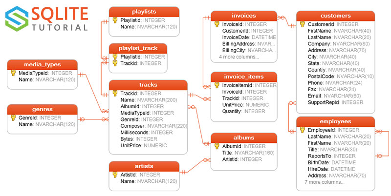
Chinook database tables and their relationships (source: https://www.sqlitetutorial.net/sqlite-sample-database/)

The Chinook sample database contains 11 tables, as follows:

Table	Purpose	Relationships
`employees`	Employee records and org hierarchy	Self-reference: `Employees.ReportsTo → Employees.EmployeeId`
`customers`	Customer profiles and contact info	`Customers.SupportRepId → Employees.EmployeeId`
`invoices`	Invoice headers (who/when/where, totals)	`Invoices.CustomerId → Customers.CustomerId`
`invoice_items`	Line items belonging to invoices	`InvoiceItems.InvoiceId → Invoices.InvoiceId`; `InvoiceItems.TrackId → Tracks.TrackId`
`artists`	Catalog of artists	1→N with `Albums`: `Albums.ArtistId → Artists.ArtistId`
`albums`	Album metadata (collections of tracks)	`Albums.ArtistId → Artists.ArtistId`; 1→N with `Tracks`
`media_types`	Media encoding types (e.g., MPEG, AAC)	Referenced by `Tracks.MediaTypeId → MediaTypes.MediaTypeId`
`genres`	Music genres (rock, jazz, metal, …)	Referenced by `Tracks.GenreId → Genres.GenreId`
`tracks`	Song/track catalog	`Tracks.AlbumId → Albums.AlbumId`; also → `MediaTypes`, `Genres`
`playlists`	Playlists container	M:N with `Tracks` via `PlaylistTrack`
`playlist_track`	Join table for playlists ↔ tracks	`PlaylistTrack.PlaylistId → Playlists.PlaylistId`; `PlaylistTrack.TrackId → Tracks.TrackId`

Exercise Codes

Open notebook: click me

Regression Preview

What is Regression?

Regression is one of the simplest machine learning algorithms.

Its goal is to predict a continuous output variable (y) from one or more input variables (X).

Common examples include:

Study hours → Exam scores
Advertising expenses → Sales revenue

The mathematical form of a simple linear regression model is:

\[ y = \beta_0 + \beta_1 x + \epsilon \]

where:

\( y \): dependent variable (target to predict)
\( x \): independent variable (input feature)
\( \beta_0 \): intercept (constant term)
\( \beta_1 \): slope (effect of x on y)
\( \epsilon \): error term

Using Pandas with Other Libraries

One of the biggest strengths of Pandas is that it integrates seamlessly with other Python libraries such as NumPy and scikit-learn (sklearn).

With NumPy, we can easily perform numerical operations, fit simple regression lines, and calculate error metrics.
With scikit-learn, we can build more advanced regression models, evaluate them with standard tools, and extend to more complex machine learning workflows.

This integration makes Pandas a central hub for managing datasets before passing them to numerical or machine learning packages.

Example: Regression with NumPy

import numpy as np
import pandas as pd
import matplotlib.pyplot as plt

# Sample data
hours = np.array([1,2,3,4,5,6,7,8,9,10])
scores = np.array([50,55,60,65,70,72,75,78,82,85])

# Fit a regression line using NumPy
coef = np.polyfit(hours, scores, 1)  # slope, intercept
line = np.poly1d(coef)

plt.scatter(hours, scores, label="Data")
plt.plot(hours, line(hours), color="red", label="Regression line")
plt.xlabel("Study Hours")
plt.ylabel("Exam Score")
plt.legend()
plt.show()

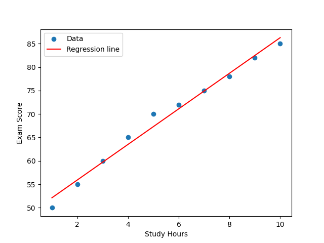
In this example, we used NumPy to fit a simple regression line between study hours (X) and exam scores (y). The function np.polyfit(hours, scores, 1) calculated the slope and intercept of the best-fitting line.

Scatter Plot of Data The scatter plot shows each student’s study hours on the x-axis and exam scores on the y-axis. As expected, there is a clear upward trend: students who studied more hours generally achieved higher scores.
Regression Line The red regression line represents the predicted relationship. It is drawn based on the slope and intercept computed by NumPy. The positive slope indicates a positive correlation: as study hours increase, exam scores also rise.
Interpretation
- The slope value (β₁) tells us how many additional points in the exam score are expected for each extra hour of study.
- The intercept (β₀) represents the predicted exam score when study hours = 0.
- Together, these values give us a simple but useful model to estimate exam performance from study time.

Example: Regression with scikit-learn

import pandas as pd
import numpy as np
import matplotlib.pyplot as plt
from sklearn.linear_model import LinearRegression

# Sample data
hours = np.array([1,2,3,4,5,6,7,8,9,10]).reshape(-1,1)  # X must be 2D for sklearn
scores = np.array([50,55,60,65,70,72,75,78,82,85])

# Create a Pandas DataFrame
df = pd.DataFrame({"hours": hours.flatten(), "scores": scores})

# Build and fit a linear regression model
model = LinearRegression()
model.fit(df[["hours"]], df["scores"])

# Predict values
pred = model.predict(df[["hours"]])

# Display coefficients
print("Intercept:", model.intercept_)
print("Slope:", model.coef_[0])

# Plot regression line
plt.scatter(df["hours"], df["scores"], label="Data")
plt.plot(df["hours"], pred, color="green", label="Sklearn Regression line")
plt.xlabel("Study Hours")
plt.ylabel("Exam Score")
plt.legend()
plt.show()

Intercept: 48.33333333333333
Slope: 3.793939393939395

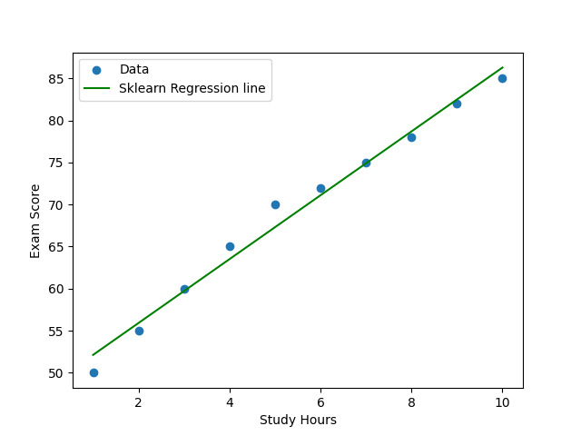
This example shows how Pandas works smoothly with scikit-learn. We can use Pandas DataFrames as inputs to fit() and predict(), making the workflow much simpler and more intuitive.

Evaluating Prediction Performance

We can measure how well the regression line fits the data using Mean Squared Error (MSE).

# Predictions from the regression line
pred = model.predict(df[["hours"]])

# Calculate Mean Squared Error
mse = np.mean((df["scores"] - pred)**2)
print("MSE:", mse)

MSE: 1.809696969696968

A smaller MSE value indicates a better fit between the model and the data.

Homeworks

This assignment reinforces your understanding of Pandas data manipulation, database handling, and basic regression concepts.

Homework 1 — Grouping and Aggregation

Create a DataFrame named sales with the following columns:

region	department	sales
East	HR	2000
East	IT	2500
West	HR	2200
West	IT	2700
South	HR	2100
South	IT	2600

👉 Using groupby(), calculate:

The average sales per region.
The total sales per department.

Explain the difference between .mean() and .sum() when applied after groupby().

Homework 2 — Combining DataFrames

Given two tables:

employees = pd.DataFrame({
    "EmpID": [1,2,3,4],
    "Name": ["Alice","Bob","Charlie","David"]
})

salaries = pd.DataFrame({
    "EmpID": [2,3,4,5],
    "Salary": [5000,6000,5500,4500]
})

Perform the following:

Merge the two DataFrames using different how options (inner, left, outer).
Explain how the result differs for each type of join.

Homework 3 — Pivot Table

Create a DataFrame with columns:
team, year, and score, similar to the pivot example in the lecture.

Then:

Build a pivot table showing the average score per team per year.
Include total averages using margins=True and name the totals row “Overall”.
Discuss how pivot_table differs from groupby().

Homework 4 — Regression Practice

Using the following data:

Study Hours	Exam Score
1	50
2	55
3	60
4	65
5	70
6	72
7	75
8	78
9	82
10	85

Perform the following:

Fit a simple regression line using NumPy (np.polyfit).
Plot the line and data points using Matplotlib.
Interpret the slope (β₁) and intercept (β₀) in your own words.
Verify the statement:

“As the number of study hours increases, the exam score also increases.”

← Pandas Basics Model Performance Evaluation →

Pandas Applications and Regression Preview

Pandas Applications and Regression Preview

Learning Objectives

Pandas Applications

Grouping and Aggregation

What is groupby()?

Pandas groupby with Multiple Columns

Applying Aggregation with agg()

Without groupby()

Custom Aggregation

Combining DataFrames

merge()

concat()

join()

When to Use Each Method

Practical Tips

Excercise

Pivoting

Core Syntax

Key Parameters

Exercise

Working with Database Files

What is SQL (Structured Query Language)

Create a sample SQLite database file

Read data from the database using pandas

Modify and save the DataFrame back into the database

Actual Practice using Real Data

Regression Preview

What is Regression?

Using Pandas with Other Libraries

Example: Regression with NumPy

Example: Regression with scikit-learn

Evaluating Prediction Performance

Homeworks

Homework 1 — Grouping and Aggregation

Homework 2 — Combining DataFrames

Homework 3 — Pivot Table

Homework 4 — Regression Practice

What is `groupby()`?

Pandas `groupby` with Multiple Columns

Applying Aggregation with `agg()`

Without `groupby()`

`merge()`

`concat()`

`join()`